Settings in General Diffusion Simulation
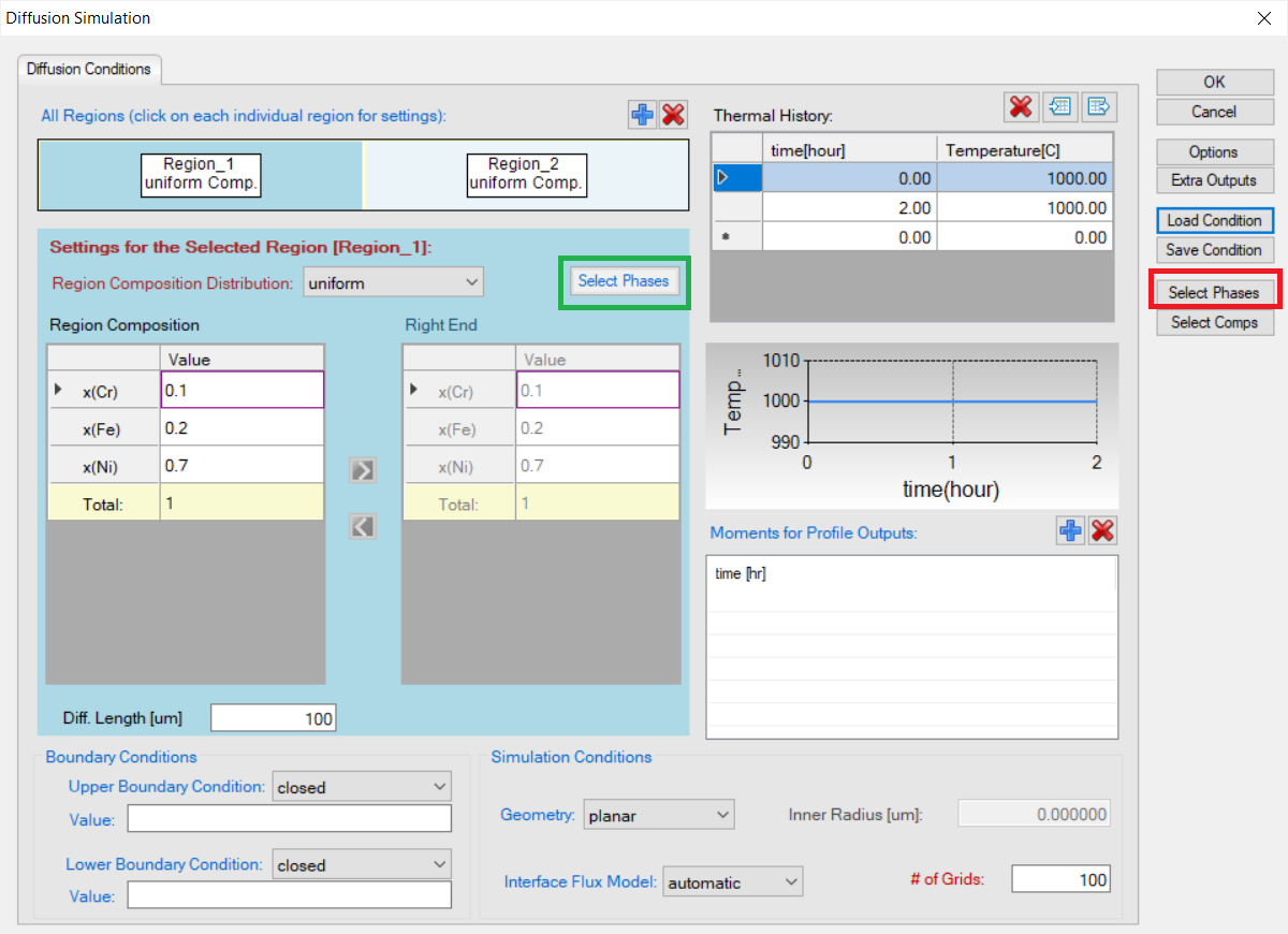
User can perform variety of diffusion simulations by PanDiffusion module. All types of simulations, except for particle dissolution, share the same general graphic user interface (GUI) to set up simulation conditions. This GUI can be accessed through the menu bar "PanDiffusion→ Diffusion Simulation", or by clicking ![]() on the Toolbar. Figure 1 shows the GUI interface of general diffusion simulation.
on the Toolbar. Figure 1 shows the GUI interface of general diffusion simulation.
Set Units
In the GUI of PanDiffusion, unit settings can be accessed through “Options → Calculation → Units”. Please refer to Section Options for details.
Select Phases
By clicking “Select Phases” as highlighted by the red box in Figure 1, user can select phases involved in the diffusion simulation on the system level. By default, all the phases in the alloy system are selected, while user can deselect some of them as wishes. In addition, user can also select phases for each region by clicking “Select Phases” as highlighted by the green box in Figure 1. By default, phase selection for each region follows the global setting in the system level.
Set Initial Composition Profile
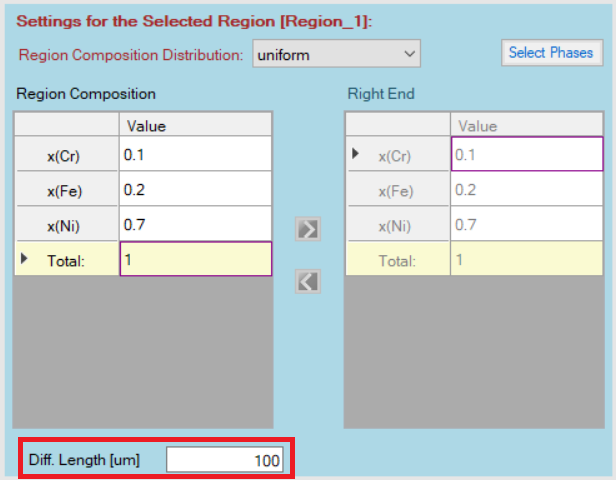
In the GUI of PanDiffusion, initial composition profile is assigned region-by-region. In each region, composition profile can be:
-
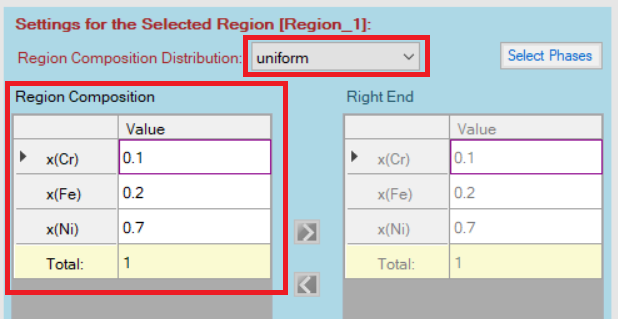
Uniform: the composition of each element in the selected Region is a constant. When “uniform” is selected, a homogenous “Region Composition” can be set.
-
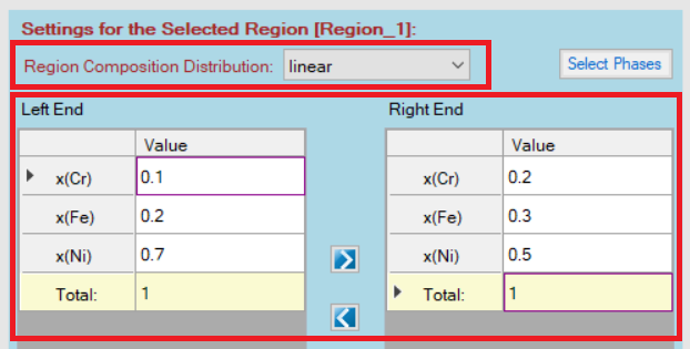
Linear: a linear composition interpolation is set from the left edge to the right edge of the selected Region. When “linear” is selected, both “Left End” and “Right End” compositions need to be set.
-
Input_file: Load composition profile from a tab-delimited .dat (or .txt) file with the following two kinds of formats:
Format (I): the distance is specified for each element, which is usually the case when using experimental data. The 1st row contains the name of each column, the 2nd row contains the unit definition, and value starts from the 3rd row.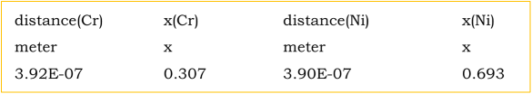
Format (II): the distance is specified in the 1st column, the composition of every element correspond to the same distance. This format is usually obtained by digitizing data from literature. The 1st row contains the name of each column, the 2nd row contains the unit definition, and value starts from the 3rd row.

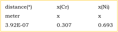
The unit of distance can be: meter (or m), millimeter (or mm), micrometer (or um), nanometer (or nm) and angstrom (Å). The unit of composition can be: x for mole fraction, x% for mole percentage, w for weight fraction, and w% for weight percentage. Note that, the units in the input file will override setting in “Options → Calculation → Units” and the input file is case insensitive.
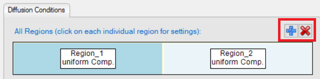
Delete or Add a Region
In the GUI of PanDiffusion, there are two Regions by default. In the following cases, single region is recommended:
-
Only one input composition profile
-
Carburization, decarburization, or other surface flux process, with a homogeneous initial composition profile
-
Homogenization of a linear composition profile
The redundant region can be removed by first selecting the Region, then clicking ![]() button as shown in . If diffusion is among three or more Regions, Regions can also be added one by one by clicking
button as shown in . If diffusion is among three or more Regions, Regions can also be added one by one by clicking ![]() .
.
Set Regional Length
In the GUI of PanDiffusion, “Diff. Length” is the length of a region.
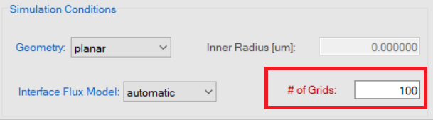
Set # of Grids
In the GUI of PanDiffusion, number of grids is set for the entire simulation box and is distributed automatically to each region.
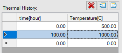
Set Thermal History
In the GUI of PanDiffusion, “Thermal History” controls temperature and the duration at each temperature. The setting in Figure 7 indicates that the temperature increases linearly from 500°C to 1000°C by 100 hours (5°C/hour).
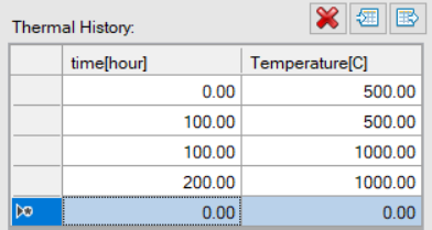
The setting shown in Figure 8 means that the sample is held at 500°C for 100 hours, and then the furnace temperature is suddenly increased to 1000°C and held there for another 100 hours.
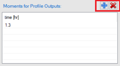
Add Moments for Profile Outputs
For a calculation set up through GUI of PanDiffusion, two moments of profiles, initial and final, will be provided by default. To add more intermediate moments of profiles, click ![]() besides the “Moments for Profile Outputs”, and edit time of the expected moment.
besides the “Moments for Profile Outputs”, and edit time of the expected moment.
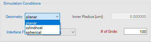
Set Geometry
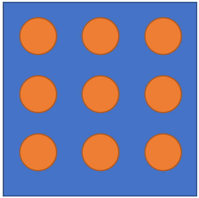
In the GUI of PanDiffusion, “Geometry” under “Simulation Conditions” decides the shape of inter-grid interface. By default, “planar” is used for most diffusion couple simulations. When particle homogenization or transformation is performed, “spherical” or “cylindrical” could be selected depending on the problem of interest.
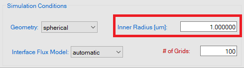
Set Inner Radius
When geometry other than “planar” is selected, user can set inner radius of cell, to simulate for a tube or shell geometry. When “cylindrical” geometry is selected, and the inner radius is non-zero, tube geometry is set up. When “spherical” geometry is selected, and the inner radius is non-zero, shell geometry is set up.
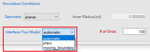
Set Interface Flux Model
In the GUI of PanDiffusion, “Interface Flux Model” under “Simulation Conditions” decides how the grid composition evolves at the interface between different phases. The option “automatic” is selected by default, which chooses the interface flux model automatically based on the number of phases selected in each region. When “plain” is selected, the mobility of the solute elements is determined by the weighted average of the mobilities of the individual phases occurring in a grid point (See the Section Set Effective Mobility (Advanced option)). When "moving_boundary" is selected, a sharp interface model is used to calculated the flux across the phase boundary which does not require the effective mobility.
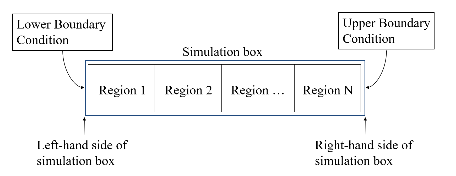
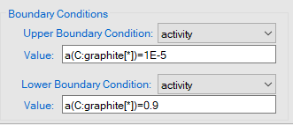
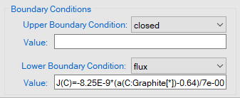
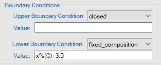
Set Boundary Conditions
There are “Upper Boundary Condition” and “Lower Boundary Condition” in PanDiffusion. Their definitions are illustrated in the following figure:
-
Fixed activity at boundaries can be set following the format:
-
Mass flux expression at boundaries can be set following the format:
-
Fixed composition of boundaries can be set following the format:
Set Effective Mobility (Advanced option)
If the “ Interface Flux Model ” chosen is “plain”, then the choice of the effective mobility determines the flux across the interface. More details about the various effective mobilities definition can be found in [2009Lar] The default choice for the effective mobility is “HS_lower”. It would be mentioned in the input batch file as shown below.
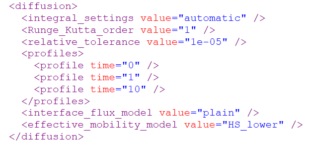
Based on the expected distribution of phases within the grid point, the effective mobility should be chosen as shown in the table below. Sometimes, the user may not know the choice between “HS_upper” and “HS_lower” as they don’t know the mobility of individual phases. In such cases, they can use the option “HS_matrix:YYY” where YYY is the expected matrix phase (i.e. the connected phase) in the microstructure. Additionally, "H_major” option is also available where the majority phases will be considered as the connected phase.


[2009Lar] H. Larsson, L. Höglund, Multiphase diffusion simulations in 1D using the DICTRA homogenization model, Calphad, 33 (2009) 495-501.